Throw a ball, fire a cannon, or launch a soccer kick, and the resulting path is a parabola — one of the cleanest and most useful results in introductory mechanics. Projectile motion is popular in physics courses for good reason: it needs nothing more than constant-acceleration kinematics, yet it produces a rich, testable, visually intuitive result.
The key idea: decompose into two independent problems
The entire trick to projectile motion is recognizing that horizontal and vertical motion don’t affect each other. Ignoring air resistance, the only force acting on a projectile mid-flight is gravity, which points straight down. That means:
- Horizontally, there’s no force at all, so velocity is constant:
- Vertically, gravity produces constant downward acceleration:
Two easy, independent 1-D kinematics problems, glued together only by a shared time variable .
Setting up the equations
If a projectile launches with initial speed at angle above the horizontal, the initial velocity components are:
Position as a function of time then follows directly from constant-acceleration kinematics:
Everything else — range, maximum height, time of flight — falls out of these two equations.
Time of flight and maximum height
Setting (assuming launch and landing at the same height) and solving for the nonzero root gives the total time in the air:
The projectile reaches its peak at exactly half that time, when :
The range equation
Plugging the time of flight into gives the horizontal range:
(using the identity ). This single equation explains a well-known result: since is maximized when , the range is greatest at a 45° launch angle — and, notably, gives the same value for complementary angles like 30° and 60°, so those two angles produce identical range, just with very different trajectories (one flat and fast, one high and slow).
Eliminating time: the trajectory equation
Solving the equation for and substituting into eliminates the time variable entirely, giving directly as a function of :
This is manifestly a parabola — a quadratic in — which is why every idealized projectile path looks the same geometric shape, just stretched or compressed depending on and .
Simulating it directly
The equations above are exact for the idealized case, but it’s often more flexible to simulate the motion step by step, which also makes it trivial to add complications like drag later. A minimal Euler-integration loop looks like this:
const g = 9.81; // m/s^2
let vx = v0 * Math.cos(theta);
let vy = v0 * Math.sin(theta);
let x = 0, y = 0;
const dt = 0.01;

while (y >= 0) {
  x += vx * dt;
  y += vy * dt;
  vy -= g * dt;
}

console.log(`Landed at x = ${x.toFixed(2)} m`);
This is exactly the kind of numerical integration that underlies real physics engines — instead of solving the closed-form equations, you advance position and velocity by small time steps, which generalizes far better once forces stop being constant.
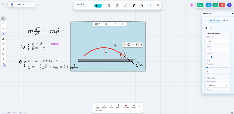
Try different angles side by side: the cleanest way to see how launch angle and initial speed trade off is to launch several projectiles at once and compare their paths. SimuBoard’s mechanical simulation engine renders the trajectory live on an infinite whiteboard, so you can adjust the angle, watch the parabola reshape in real time, and directly compare range and max height across launches.
Where the idealized model breaks down
Real trajectories deviate from this clean parabola for a few reasons:
- Air resistance — drag scales with velocity squared for most projectiles at everyday speeds, which breaks the clean analytic solution and requires numerical integration (like the loop above) to solve.
- Spin — a spinning ball experiences the Magnus effect, curving its path sideways — the basis of curveballs, banana kicks, and swing bowling.
- Variation in — over very long ranges (artillery, ballistic missiles), the assumption of constant, uniform gravity starts to break down.
Even with those complications, the idealized parabola remains the right starting point: it’s the zeroth-order approximation that every more realistic model is built on top of.